Maximum Cut and the Goemans–Williamson Algorithm

Given a graph $G(V,E)$, which we will refer to simply as $G$, consider partitioning the vertex set $V$ into two disjoint sets $A$ and $B$, and counting the number of edges $e_k=(v_i,v_j)$ where $v_i\in A$ and $v_j\in B$.

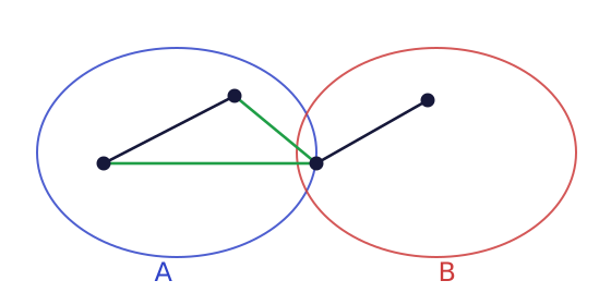
For this partition we have two edges crossing between $A$ and $B$. Is it possible to have more? For an arbitrary graph $G$, can we maximize the number of edges that cross from $A$ to $B$, and identify the partition(s) that attain it? This is the maximum cut problem. The size of a cut is the number of edges crossing between $A$ and $B$, and the maximum cut is a cut with at least as many edges as every other cut.

An NP-complete problem

The maximum cut problem is known to be NP-complete; in fact, it was one of Karp's original 21 NP-complete problems.

A quadratic reformulation

The adjacency matrix $A_G$ has entry $a_{ij}$ equal to $1$ when there is an edge between $v_i$ and $v_j$, and $0$ otherwise. Now rewrite the max cut as a quadratic program. Assign every vertex in $A$ the value $1$ and every vertex in $B$ the value $-1$, so a partition becomes a choice of $x_i\in\{-1,1\}$ at each vertex. Then

Every crossing edge contributes $a_{ij}(1-x_i x_j)=2$, and since the $(i,j)$ and $(j,i)$ terms agree we quadruple-count the cut, which is where the factor of $\tfrac14$ comes from.

A cut for free

It is easy to find a cut of any graph that attains at least half of the max cut. Writing $\#E(A,B)$ for the number of edges in the cut of a partition $V=A\cup B$, there is always a partition with

A random split already achieves this in expectation, since each edge crosses with probability $\tfrac12$. The Edwards–Erdős bound sharpens it: every graph with $m$ edges has a cut of size at least

and this is tight for complete graphs.

Max cut on special graphs

For some families the maximum cut is known exactly. A complete graph on $2m$ vertices has maximum cut $m^2$, attained by splitting the vertices as evenly as possible; the proof is the simple inequality $m^2 > j(2m-j)$ for any uneven split. And a tree with $m$ edges has maximum cut exactly $m$: a tree has no cycles, so it is bipartite, and the two-coloring puts every edge across the cut.

The Goemans–Williamson algorithm

To do better in general, we relax the quadratic program. Instead of forcing each $x_i\in\{-1,1\}$, let each vertex be a unit vector and maximize

This is a semidefinite program, and unlike the original it can be solved in polynomial time.

But a solution to the semidefinite program is a list of $n$ vectors in $\mathbb{R}^n$, not a cut of our graph. Surprisingly, the most difficult part of using this relaxation is translating the result back into a meaningful cut. The key idea is randomized hyperplane rounding: round each vector to $1$ or $-1$ depending on which side of a random hyperplane it lands on.

To choose the hyperplane, sample $n$ independent standard normal variables $y_1,\dots,y_n$ and normalize $\vec n = (y_1,\dots,y_n)/\lVert(y_1,\dots,y_n)\rVert$ to get its normal direction.

Taking expectations and using that bound on every edge gives the Goemans–Williamson guarantee: the expected size of the resulting cut is at least

So the algorithm always lands within about $88\%$ of the best possible cut: a hard guarantee, on every graph, in polynomial time. Under the unique games conjecture no efficient algorithm can beat this constant, which ties $0.878$ back to the $P = NP$ question it started from.

Max cut turns up across theoretical computer science, network design, machine learning, and even theoretical physics, and the tools behind it (semidefinite programming, randomized rounding, and the probabilistic method) reach much further than this one problem. The full paper can be found here.