Haar Graphs | Austin Ulrigg

Keine Sorge, meine deutschen Leser, hier geht es nicht um Haare oder das Hairy-Ball-Theorem.

Seven graph theorists want to meet for coffee. They agree to meet three at a time and, naturally, require every pair to meet exactly once. The task that remains is deciding who should attend which meetings in order to achieve this.

Each meeting uses three of the $\binom{7}{2}=21$ pairs, so there must be seven meetings. Each person has six others to meet, two at a time, so everyone must attend three meetings.

One way to ensure that everyone attends three meetings is to number the people $0,1,\ldots,6$ around a circle, choose a triple, and move all three choices one place clockwise for each of the next six meetings. In other words, add $1$ to each number modulo $7$ . We only need to find a triple whose cyclic shifts never repeat a pair.

Our first guess might be $\{0,1,2\}$ . Adding $1$ gives $\{1,2,3\}$ , so people $1$ and $2$ already meet twice.

Any two names are one, two, or three steps apart around the circle, counting in whichever direction is shorter. The seven cyclic shifts of a pair give all seven pairs at that distance. So, if the three pairs in our triple have different distances, no pair will repeat. The triple $\{0,1,3\}$ does this. The names $0$ and $1$ are one step apart, $1$ and $3$ are two, and $0$ and $3$ are three.

Mohar, Erdős, Steinerberger, Ringel, Youngs, Pisanski, and Euler are numbered 0 through 6 around a circle. The first meeting selects 0, 1, and 3. Moving all three choices one place clockwise selects 1, 2, and 4. — Figure 1. The first meeting and its first cyclic shift.

The seven meetings are then

\begin{gathered} \{0,1,3\},\quad\{1,2,4\},\quad\{2,3,5\},\quad\{3,4,6\},\\ \{4,5,0\},\quad\{5,6,1\},\quad\{6,0,2\}. \end{gathered}

Because they are graph theorists, they want to record attendance in a graph. Thus, we make a vertex $A_i$ for meeting $\{i,i+1,i+3\}$ and a vertex $B_j$ for person $j$ . Join them when person $j$ attends meeting $i$ , taking subscripts modulo $7$ . The resulting graph is called the Heawood graph.

The Heawood graph. Solid vertices represent meetings and hollow vertices represent people, with the seven graph theorists names beside their B labels. A_i is joined to B_i, B_(i+1), and B_(i+3), modulo 7. — Figure 2. The graph of our seven meetings.

Each meeting has three people and each person attends three meetings, so every vertex has degree three. The graph is bipartite, with meetings in one class and people in the other. In terms of the coffee problem, if there were a four-cycle then this would mean two people attended the same two meetings.

We have been adding modulo $7$ , so our labels belong to the cyclic group $\mathbb Z_7$ . The edges of the graph are determined entirely from the set $S=\{0,1,3\}$ , using the rule

A_i\sim B_j\quad\Longleftrightarrow\quad j-i\in S.

We chose $S$ to solve the coffee problem. But if we are just interested in the graph,¹ could we do this for any subset $S$ ? And could we replace $\mathbb Z_7$ by a different group? As you might've guessed since you are reading this post, it turns out this construction works for any finite group.

For a finite group $\Gamma$ and a subset $S\subseteq\Gamma$ , make two disjoint sets of vertices

\{A_g\mid g\in\Gamma\}\ \cup\ \{B_g\mid g\in\Gamma\},

and join $A_g$ to $B_{gs}$ for each $s\in S$ . This is the Haar graph $H(\Gamma,S)$ , and $S$ is its connection set. Equivalently, $A_g\sim B_{g'}$ exactly when $g^{-1}g'\in S$ . In an additive group, this becomes $g'-g\in S$ , so our example is $H(\mathbb Z_7,\{0,1,3\})$ . When $\Gamma$ is cyclic, these are called cyclic Haar graphs.

Each label $s$ gives one edge at every vertex, connecting $A_g$ to $B_{gs}$ and $B_g$ to $A_{gs^{-1}}$ . Thus, the graph is simple, bipartite, and $|S|$ -regular, with $2|\Gamma|$ vertices and $|\Gamma||S|$ edges. The edges of any one label correspond to a perfect matching, as the colors in Figure 2 show.

Hladnik, Marušič, and Pisanski studied these graphs for abelian groups in Cyclic Haar graphs (2002). Estélyi and Pisanski later considered arbitrary finite groups in Which Haar graphs are Cayley graphs? (2016).

Adding $1$ modulo $7$ to every subscript takes an edge such as $A_0B_3$ to $A_1B_4$ . Any such map preserves vertex adjacency, giving an automorphism. We can do the same thing in any Haar graph. Left multiplication by $h\in\Gamma$ sends

A_gB_{gs}\longmapsto A_{hg}B_{hgs}=A_{hg}B_{(hg)s}.

Exactly one left multiplication takes $A_g$ to a given $A_{g'}$ , namely multiplication by $g'g^{-1}$ . The same holds in the $B$ -class. We say that $\Gamma$ acts simply transitively, or regularly, on each class.

We can also use this observation in reverse. Suppose a bipartite graph has a group $\Gamma$ acting by automorphisms, simply transitively on each class. Choose a vertex $A$ in one class and $B$ in the other. Every vertex then has a unique label $A_g=gA$ or $B_g=gB$ . Take $S$ to consist of the elements $s$ for which $A\sim sB$ . Applying $g^{-1}$ shows that $gA\sim g'B$ exactly when $g^{-1}g'\in S$ . Thus, the graph is $H(\Gamma,S)$ .

The choice of $S$ also affects whether the graph is connected. To reach another $A$ -vertex, we first follow an edge labeled $s$ to the $B$ -class, then return along one labeled $t$ , giving

A_g\longrightarrow B_{gs}\longrightarrow A_{gst^{-1}}.

Repeating these pairs of steps from $A_{1_\Gamma}$ reaches exactly the $A$ -vertices indexed by the subgroup generated by $SS^{-1}=\{st^{-1}\mid s,t\in S\}$ . Thus, for nonempty $S$ , the graph is connected exactly when $SS^{-1}$ generates $\Gamma$ . If $1_\Gamma\in S$ , this is equivalent to $S$ generating $\Gamma$ . The Heawood graph is connected because $S$ contains $0$ and the generator $1$ .

The edge labels are also useful when building a rotation system. Choose a cyclic order $\alpha$ on $S$ and order the edges at every $A$ -vertex by their labels. Each label occurs on exactly one incident edge, so this gives a local rotation. Do the same at the $B$ -vertices with another order $\beta$ , and we have a rotation system. Left multiplication preserves each edge label, taking $A_gB_{gs}$ to $A_{hg}B_{(hg)s}$ , so it also preserves these orders.

Our graph has fourteen vertices, each with two possible cyclic orders. That gives $2^{14}$ rotation systems if we choose the orders separately. But if we use $\alpha$ at every $A$ -vertex and $\beta$ at every $B$ -vertex, there are just two choices for each, giving four rotation systems to try.

We can keep track of these orders on a much smaller graph, with one vertex $A$ , one vertex $B$ , and one edge for each $s\in S$ . This graph of parallel edges is a dipole, with the orders $\alpha$ and $\beta$ at its two vertices.

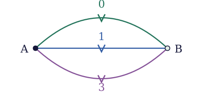
A dipole with vertices A and B and three parallel edges directed from A to B, labeled 0, 1, and 3 in Z7. — Figure 3. The dipole for $S=\{0,1,3\}$ .

Figure 3 is an example of a voltage graph. The smaller graph is called the base graph. Choose a direction for each of its edges and label it with an element of a group $\Gamma$ . This label is the voltage. Reading an edge in the opposite direction replaces its label by its inverse. In an additive group, it changes the sign.

To build the derived graph, make a copy $u_g$ of each base vertex $u$ for every $g\in\Gamma$ . An arrow $u\to v$ with voltage $s$ gives an edge $u_gv_{gs}$ for each $g$ . Thus, the label tells us which copy of $v$ to join to a given copy of $u$ . For our dipole, the labels $0$ , $1$ , and $3$ give the three colored matchings in Figure 2. A Haar graph is exactly the derived graph of a dipole with one voltage for each element of $S$ .

A base edge from A to B with voltage 1 in Z7 gives seven derived edges from A_i to B_(i+1). The B vertices carry the seven graph theorists names beside their numbers. — Figure 4. One voltage gives a perfect matching.

We can also choose rotations at the base vertices. Each copy then gets the same cyclic order of the corresponding edge ends. For our dipole, these are the two orders $\alpha$ and $\beta$ .

A walk in the base graph determines a walk in the derived graph once we choose a copy of its starting vertex. This is called a lift. For example, take edge $0$ forward and edge $1$ backward in the dipole. The backward step contributes $-1$ . The base walk returns to $A$ , but its lift from $A_0$ ends at $A_6$ .

A closed base walk takes edge 0 from A to B and edge 1 backward from B to A. Its signed voltages are 0 and minus 1. The lifted walk goes from A0 to B0, named Mohar, and ends at A6 rather than A0. — Figure 5. A closed base walk whose lift does not close.

Each pair of steps subtracts $1$ modulo $7$ , so seven repetitions give a fourteen-cycle. More generally, multiply the voltages along a walk in the order they are encountered, using inverses when traveling backward. This product is its net voltage. A closed base walk lifts to a closed walk exactly when its net voltage is the identity. For additive groups, we add the labels instead.

A current graph starts with an embedded graph whose directed edges have group labels, called currents. Reversing an edge inverts its current. For example, take the dipole below, with currents $1$ , $2$ , and $4$ in $\mathbb Z_7$ , all directed from $u$ to $v$ . The cyclic order $(1\ 2\ 4)$ at both vertices specifies an orientable cellular embedding.

A current graph with currents 1, 2, and 4 directed from u to v in Z7. Both vertices have cyclic order 1, 2, 4. Tracing its single face reads 1, minus 2, 4, minus 1, 2, minus 4. — Figure 6. The rotations specify a single face.

We can trace a face by starting with edge $1$ from $u$ to $v$ . The rotation at $v$ tells us to take edge $2$ next, which brings us back to $u$ . At $u$ , edge $4$ comes next, so we follow it to $v$ . Continuing in this way, we read $1,-2,4,-1,2,-4$ before returning to the dart we started with. Since we have used every edge in both directions, the embedding has only one face.

Figure 7(a) shows this face cut open into a hexagon. Put a new vertex $f$ inside it and join $f$ to the middle of each side. There are six sides in the picture because each of the three original edges appears twice along the boundary. In particular, the sides marked $1$ and $-1$ both come from edge $1$ . Gluing them back together joins the two segments into a single edge from $f$ to itself, crossing edge $1$ . Each of the other two pairs gives a loop in the same way, leaving one vertex and three loops. This gives the dual of the original embedding.

The current graph's single face is cut open into a hexagon with successive labels 1, minus 2, 4, minus 1, 2, minus 4. Six colored segments connect a new vertex f to the sides. Joining each pair of sides with opposite labels connects its two segments into one loop at f. The three resulting loops appear on the right. — Figure 7. From the current graph to its dual.

Now give these loops voltages $1$ , $2$ , and $4$ , with the directions shown in Figure 7(b). For the green loop, leaving $f$ along the upper segment follows the arrows and gives voltage $1$ . Leaving along the lower segment goes around the same loop backward and gives voltage $-1$ . Reading the signed labels clockwise around $f$ gives $1,-2,4,-1,2,-4$ , in the same order as around the original face.

The voltage construction replaces $f$ by seven vertices $f_0,\ldots,f_6$ , which we'll just call $0,\ldots,6$ . The loop with voltage $1$ gives an edge from $i$ to $i+1$ for every $i$ , modulo $7$ . For $i=0$ this joins $0$ to $1$ , and for $i=6$ it joins $6$ to $0$ . Thus $0$ has neighbors $1$ and $6$ from this loop. The loop with voltage $2$ gives it neighbors $2$ and $5$ , and the loop with voltage $4$ gives it neighbors $4$ and $3$ . In the cyclic order from Figure 7(b), these neighbors occur as $(1\ 5\ 4\ 6\ 2\ 3)$ . At vertex $i$ , we add $i$ to each entry, giving

(i+1,\ i+5,\ i+4,\ i+6,\ i+2,\ i+3).

Two local rotations of the derived K7, centered at the numbers 0 and 1. Names appear beside the neighboring vertices. At 0 the clockwise neighbors are 1, 5, 4, 6, 2, 3. At 1 they are 2, 6, 5, 0, 3, 4. Adding 1 to every label gives the second rotation. — Figure 8. Adding $1$ to every label gives the next rotation.

Each vertex is adjacent to all six others, so the derived graph is $K_7$ . We can trace one of its faces directly. Start with $0\to1$ . In the rotation at $1$ , the neighbor after $0$ is $3$ , so next we take $1\to3$ . At $3$ , the neighbor after $1$ is $0$ , and at $0$ , the neighbor after $3$ is $1$ . We have returned to the starting dart after tracing the triangle $0,1,3,0$ .

The changes in vertex label along this triangle are $1,2,4$ , the currents leaving $u$ in their cyclic order. In the dual embedding, there is a face containing $u$ . Its boundary crosses the three original edges at $u$ , traversing the loops with voltages $1,2,4$ . Since we copied the dual rotations, following this boundary in the derived graph gives the same increments. Their sum is $0$ modulo $7$ , so three steps return us to our starting vertex. At $v$ , the outgoing currents are $-1,-2,-4$ , which also sum to $0$ and give the triangle $0,6,4,0$ . The condition that the outgoing currents sum to $0$ at each vertex is called Kirchhoff's current law.

Two triangular faces in the derived K7. The first goes from 0 to 1 to 3 and back to 0, using increments 1, 2, 4. The second goes from 0 to 6 to 4 and back to 0, using increments minus 1, minus 2, minus 4. — Figure 9. Kirchhoff's law closes both triangles modulo $7$ .

Adding each element of $\mathbb Z_7$ to the vertex labels gives seven triangles of each kind. These are the fourteen faces. So this two-vertex current graph has given us a triangular embedding of $K_7$ .

William Sharp Gustin, an American mathematician, developed the current-graph method in 1963, and it became central to Ringel and Youngs's 1968 solution of the orientable Heawood map-coloring problem. Gross (1974) introduced voltage graphs as a dual approach.

Going back to our Haar graph, let's try the same cyclic order on $S=\{0,1,3\}$ at both types of vertex,

\alpha=\beta=(0\ 1\ 3).

At A_i the clockwise edge labels 0, 1, 3 lead to B_i, B_(i+1), B_(i+3). At B_i the same clockwise labels lead to A_i, A_(i-1), A_(i-3). — Figure 10. The same label order at both types of vertex.

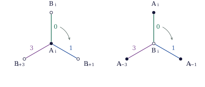
Starting with $A_0\to B_0$ , label $1$ comes next at $B_0$ , so we go to $A_{-1}=A_6$ . Label $3$ comes next at $A_6$ , taking us to $B_2$ . Following the two rotations gives the face in Figure 11.

The facial walk A0 to B0 to A6 to B2 to A2 to B3 and back to A0, with edge labels 0, 1, 3, 0, 1, and 3. — Figure 11. A facial walk of length six.

To do the same calculation for any Haar graph, write $(g,s)_A$ for $A_g\to B_{gs}$ and $(g,s)_B$ for $B_g\to A_{gs^{-1}}$ . Let $\tau$ reverse a dart and $R$ take the next dart in the local rotation. The face permutation is $F=R\tau$ , with composition read from right to left. It crosses the edge to $B_{gs}$ and takes the next label in the $B$ -rotation, giving

F(g,s)_A=(gs,\beta(s))_B.

As in our connectivity calculation, two steps bring us back to the $A$ -class. Crossing back multiplies the subscript by $\beta(s)^{-1}$ , and $\alpha$ gives the next label, so

F^2(g,s)_A=\bigl(gs\beta(s)^{-1},\alpha\beta(s)\bigr)_A.

Here, the first coordinate is the vertex subscript and the second is the label of the edge we are about to take. Returning to our starting dart means returning to the same vertex with the same edge label. Since each application of $F^2$ moves two steps along the face, a face has length four if two applications return us to the starting pair and one application does not. For every face to have length four, this must hold for every $A$ -dart. We can check this using the formula above for any choice of $\alpha$ and $\beta$ .

In our example, the edge label follows $0\to3\to1\to0$ under $\alpha\beta$ . It returns for the first time after three applications of $F^2$ , and the total change to the vertex subscript is

(0-1)+(3-0)+(1-3)=0\pmod 7.

The same calculation works starting at label $1$ or $3$ , so every face has length six. Adding each element of $\mathbb Z_7$ to all the vertex subscripts in Figure 11 gives the seven faces shown below.

The Heawood graph drawn as a hexagonal tiling inside a parallelogram. Identify opposite sides in the marked directions to form a torus. The seven faces are labeled f0 through f6, and their colors continue across the identified sides. — Figure 12. The resulting embedding, with opposite sides identified.

Because this was never really about coffee. ↩